Monday, December 14, 2015

Post 6: Raster Analysis

Goals and Objectives: 

The goal of this exercise was to use raster geoprocessing tools to create models for frac sand mining suitability and environmental and cultural risk in Trempealeau County. The results could then be overlayed to find the most desirable locations for frac sand mining with the lest impact.

Background:

Raster analysis is valuable for multiple reasons. Calculating rasters is the same as intersecting suitable vector layers. The difference with using rasters though is that you can add rasters to determine a ranking of suitability. This can be more helpful than a simple yes or no answer received from intersecting vector files. In addition, using rasters for distance analysis is more efficient than using vectors because rasters can store continuous distance information, while vectors only store discrete information.

Data Sources: 

  • Wisconsin Geological & Natural History Survey
  • U.S Department of Transportation
  • USGS National Map
    • Landcover
    • Digital Elevation Model
  • U.S. Department of Agriculture
  • Trempealeau County Land Records
  • USDA NRCS Web Soil Survey


Methods:

The entire area of Trempealeau County was too big for the raster analysis, so the southern portion of the county was used as the study area. A mask of the study area was set as the processing extent in the environmental settings.

Raster tools used include Raster Calculator, Reclassify, Euclidean Distance, Slope, Viewshed, and Focal Statistics. The equal interval classification was used for many reclasses.

Data flow models were used to create all rasters (Figures 1-3). The models are shown below:

Figure 1: The data flow model for the suitability model. Individual factors were created and classified. The factors were then combined together to create an overall suitability model.

Figure 2: The data flow model for the risk model. Individual factors were created and classified. The factors were then combined together to create an overall risk model.

Figure 3: The data flow model for creating the combined suitability/risk model. The risk model raster was multiplied by -1 so it would properly combine with the positive suitability risk raster. Both a regular and weighted suitability/risk model were created in the model. Also note the viewshed tool was run in this model to determine how visible a mine would be to a bike trial running through Perrot State Park.

Suitability rankings were assigned on a 1-3 scale, with 1=Least Suitable and 3=Most Suitable. Reasons for the rankings are discussed in the Excel table below (Figure 4). Risk rankings were assigned on a 1-3 scale, with 1=Least Risk and 3=Most Risk. Reasons for the rankings are discussed in the Excel table below (Figure 4).

Figure 4: The table shows how factors were classified and given ranks for both the suitability and risk models.

Sand Mining Suitability Model:

Criteria used in the suitability model included:
  • Geology 
  • Land Use Land Cover
  • Distance to Rail Terminals
  • Slope
  • Water Table Elevation (feet)
Specific methods for objectives in the suitability model are listed below:

Objective 4: The Slope tool was used to calculate slope based on percent rise. Raster Calculator was used to convert the DEM, which was in feet, to meters by multiplying all cells by 0.3048. The slope values were averaged using Focal Statistics, and then reclassed using the Reclassify tool based on the following parameters:

Objective 5: Depth to water table data was accessed online from the Wisconsin Geological & Natural History Survey (Wisconsin Geological & Natural History Survey, 2015).

Objectives 6 and 7: Raster Calculator was used to add all suitability classes together. This resulting in combined rankings of all factors. The factors were multiplied by the unsuitable NLCD feature class to exclude land unsuitable for mining.

Objective 14: The viewshed tool was used to determine which locations in the county were visible from a bike trail that runs through Perrort State Park. Results were ranked added to the suitability model.

Sand Mining Risk Model:

Criteria used in the risk model included: 
  • Impact to Streams
  • Impact to Prime Farmland
  • Impact to Residential Areas (Noise shed/Dust shed)
  • Impact to Schools
  • Impact to Variable of your Choice (Wildlife Areas)
Specific methods for objectives in the risk model are listed below:

Objective 8: I used streams with a ranking between 3 and 6 because they included 23% of all streams and their primary designation was Primary Flow Over Land Perennial, which means it is a river that flows more than two years. Streams ranked 2-6 included streams designations of Primary Flow Over Land Intermittent, which meant the rivers existed only some of the time. Therefore, streams ranked 2 or lower were excluded.

Objective 10: The Zoning feature class was chosen to calculate distance from residential areas. Advantages of this feature class include it had land use types, which were helpful in distinguishing were people lived. Census data would have been hard to determine congregated areas where people live. A disadvantage of using the zoning feature class was that sometimes it was hard to determine which classes were residential. For example, I used my best educated guess and determined the Incorporated class could be considered residential.

Objective 12: Wildlife Areas were chosen as risk factor because mines should not encroach upon wildlife areas.

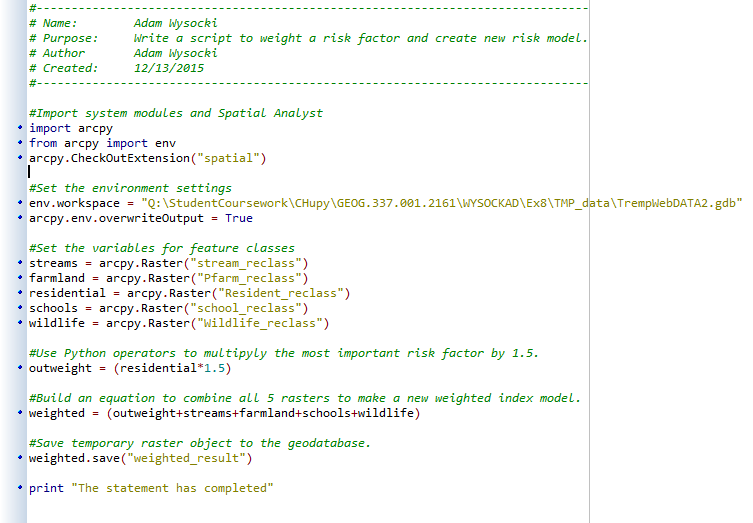
Python: Python scripting was used to weight the most important risk factor, impact to residential areas, by 1.5 (Figure 5). The results were added to the risk model, and then used to create the overall suitability/risk model (weighted).

Figure 5: The python script used raster calculator to multiply the most important mining risk factor by a weight of 1.5. The result was added to the other risk factors to create a newly weighted risk model for frac sand mining in Trempealeau County.

Overall Suitability/Risk Model: 

Raster calculator was used to combine the Mine Suitability and Mine Risk models for an overall mining suitability model. Both rasters were composed of other rasters ranked on a 1-3 scale. Raster calculator was used to convert 1-3 values of the Mine Risk model to make the values negative. When raster calculator was used to combine the models. the negative risk numbers would be added to the positive suitability numbers. This resulted in a correct Mining Suitability/Risk model. The same process was used to create a weighted mining suitability/risk model from the weighted risk model.

Results: 

Suitability Model:
Figure 6: The map shows were suitable geological formations (Jordan and Wonewoc formations), are located. All other formations are unsuitable for frac sand mining.

Figure 7: The map shows suitable land covers for mining. The more suitable locations are undeveloped and have little vegetation in the way. It should be not unsuitable land cover is listed on the map, which indicated areas populated by humans.
Figure 8: The map shows which areas of land are closer to the one rail terminal in the study area. Frac sand mines need to be close to rail terminals to ship the sand.
Figure 9: Percent slope was mapped to find areas with the lowest slope, which is most desirable for mining.

Figure 10: Water table elevations (feet) were mapped to determine where the water table was closet to the surface (most desirable).

Figure 11: All suitability factors were combined to create an overall suitability model for frac sand mining. Higher rankings are more suitable for mining.
Risk Model:

Figure 12: The map shows locations's proximity to streams. Mines closer to streams have a greater impact. 

Figure 13: The map shows where prime farmland is located. Mines on prime farmland would have a big impact.

Figure 14: The map shows proximity to residential areas. Mines closet to residential areas would have the greatest impact. Additionally, mines cannot be located within 640m of residential areas, so NoData was designated for any areas closer than 640m.

Figure 15: The map shows proximity to schools. Mines closer to schools have the greatest impact. Additionally, mines cannot be located within 640m of schools, so NoData was designated for any areas closer than 640m.
Figure 16: The map shows proximity to wildlife areas. Mines located closest to these ares would have the greatest impact.

Figure 17: All risk factors were combined to create an overall risk model for frac sand mining. Higher rankings are pose greater risk for mining.

Figure 18: The most important risk factor, impact to residential areas, was weighted by 1.5 using PyScripter. Higher rankings are areas where mines would have a greater impact.

Viewshed: Bike Trail:

Figure 19: The map shows visibility from a bike trail that runs through Perrot State Park. Establishing a mine in blue ares would keep mines out of site of the bike trail, while mining in green or brown areas would be highly visible.
Figure 20: The Bike Viewshed factor was added to the suitability model. Higher ranks are more suitable for mining (18 being the highest rank),
Overall Suitability/Risk Model:

Figure 21: The suitability model and risk model (multiplied by -1) were added to create an overall suitability/risk model for frac sand mining in Trempealeau County. Higher rankings (positive) are places more suited for mining.
Figure 22: This suitability/risk model for frac sand mining incorporated the weighted risk model in its creation. Higher rankings (positive) are places more suited for mining.

Discussion:

Large gaps in the final models can be seen (Figures 21 and 22). These are because mines cannot be within 640m of residential areas and schools, and therefore the areas were assigned NoData values.
Looking at the non-weighted suitability model, the best locations to establish frac sand mines would be in the middle of the study area indicated by spotted areas of teal (Figure 21). These areas are located further away from residential areas and schools, located on suitable geologic formations (Jordan and Wonewoc), and are located closet to the one rail terminal in the study area.

The weighted suitability model shows the bets locations to establish frac sand mines would be in the northwestern part of the study area (Figure 22). This is most likely because the risk factor "impact on residential areas" was weighted by 1.5. This shifted suitable mining areas from the middle of the study area to the northwestern area.

Overall, I believe the best location to establish a frac sand mine in this part of Trempealeau County study area would be in the northwestern part. It is close to the rail terminal, located on suitable geologic formations, and located away from residential and school areas.

Conclusion:

Raster analysis is an important tool for analyzing geographic questions. This exercise utilized many raster analysis tools to create a suitability model, risk model, and combined suitability/risk model for frac sand mining in a portion of Trempealeau County. Results indicate establishing a mine in the northwestern portion of the study area would be best. This knowledge can be used by land management officials to make informed decisions on where to mine frac sand. Knowledge of raster analysis will be very beneficial for my career in the geospatial workforce.

References:

Wisconsin Geological & Natural History Survey (2015). Generalized Water-Table Elevation Map of Trempealeau County, Wisconsin [coverage file]. Retrieved from: https://wgnhs.uwex.edu/pubs/000444/


Wednesday, November 18, 2015

Post 5: Network Analysis

Goals and Objectives:

The purpose of this lab was to conduct a network analysis to determine the economic impact of trucking sand from mines to rail terminals on local Wisconsin roads. Trempealuea County was of particular interest in the analysis. The number of truck routes and cost per mile were estimated to determine hypothetical costs of mining per county in Wisconsin. A script was created to select mines suitable for analysis. Network analysis was then used to determine the closet route from each mine to the nearest rail terminal. Using network analysis is a valuable tool that can be used by project managers to predict the costs frac sand mines will have on Wisconsin roads.

Background: 

The Midwest is home to many deposits of sand well-suited for fracking. In order to use frac sand in hydraulic fracking, the sand has to be transported from the mining site to the user. It it quite typical for mines to use rail roads to transport sand to the user. The only problem is that sand mines are usually in rural locations, and are often not near rail roads. In order to get their sand to the rail roads, mine operators will use trucks on rural roads that are not built to withstand heavy loads over long periods of time (National Center for Freight & Infrastructure Research & Educatoin, 2013). Once frac sand mines are in full swing in Wisconsin, approximately 40 million tons of sand will be transported out of Wisconsin per year (Wisconsin Department of Transportation NW Region Planning Staff, interview, May 16, 2012). In order to upkeep the roads, Wisconsin has implemented road upgrade maintenance agreements (RUMA) with frac sand mine owners. The agreements ensure mine owners pay for any repairs needed for roads their trucks drive on (National Center for Freight & Infrastructure Research & Educatoin, 2013). The suitability model we create will determine the cost of trucking sand on Wisconsin roads. This will enable land planners to make better-informed decisions on where to allow frac sand mines.

Methods: 

Data Sources:

  • Dr. Christina Hupy
  • ESRI street map USA
  • Wisconsin Department of Natural Resources


Part 1: Creating a Script

The goal for the script was to select frac sand mines suitable for network analysis in our class project, which is focused on creating a suitability model for frac sand mining in Wisconsin. These mines had to fit the following criteria:
  • Must be active 
  • Mine must not have a rail loading station. Mines with a rail loading station will use the rails to transport their sand, not the local roads. We are focused on mining's impact on local roads. 
  • Must be 1.5 km away from any rail roads. Rail road data is not totally up to date, and mines closer than 1.5 km may have had a rail spur built to them within the past few years.
Wrtiting the script used the following procedure (Figure 1): 
  • Set up the script in PyScripter
  • Set the variables for the feature classes and feature layers to be used in the exercise
  • Write 3 SQL statements to query the data based on the above criteria
  • Use the SQL statements to select the mines that meet your criteria
    • Use arcpy.MakeFeatureLayer_Management
  • Use arcpy.SelectLayerByLocation_management to 
    • Select only mines in Wisconsin
    • Remove all mines within 1.5 km of a rail line
  • Save the output layer resulting from the SQL statement using the CopyFeatures_management tool
Figure 1: The python script for this exercise used SQL statements to select frac sand mines suitable for network analysis. The SQL statement was based off three criteria listed above. 

Part 2: Network Analysis

The goal of network analysis was to find the quickest route from each frac sand mine to the nearest rail terminal. The following steps had to be taken to complete the network analysis:
  • Connect to ESRI's originalrawdata2013\streetmap_na\data
    • Add the "streets" network data set ArcMap
  • Turn on Network Analyst and open the Network Analyst toolbar
    • Make sure to turn on the Network Analyst extenstion in ArcMap
  • Add the final rail selection from the scipting portion of this exercise
  • Add the rail terminals feature class
    • Select only the terminals that have RAIL in the MODE_TYPE field. Export the selection as a feature class and add it to the map. Use these rail terminals in the analysis.
  • Use "closest facility" analysis in Network Analyst to determine which rail terminal each mine will transport its sand to and the most effecitent route between them
    • Add a new closest facility layer form the Network Analyst menu
    • Load the final mines and rail terminals into the closet facility layer
      • Incidents: mines
      • Facilities: rail terminals
    • Solve the closet facility
  • Use Model Builder to develop a data flow model that will determine the most efficient routes between each mine and the closest rail terminal
    • Before creating the model, delete the address field in the Mines final feature class (the address field causes an error in model builder)
    • Create a new tool box in your geodatabase to save the model to
    • Add the Make Closest Facility Layer tool 
      • use the Travel to facilty option in the tool
    • Use the Add Locations tool to add both the Mines and the Rail Terminals feature classes 
    • Add the Solve tool and run the model
    • Export the route that was produced from the Closet Facility Layer tool as a feature class in your geodatabase
      • Use the Select Data tool to select the route
      • Use the Copy Features tool to export the Routes feature class to your geodatabase
  • Use Model Builder to calculate the lenth of route by county and estimate the costs each county incurs in road matainanc due to trucking sand
    • Project the “Routes” output from the model to Wisconsin Transverse Mercator 1983 (WTM83)
    • Intersect the “Wisconsin Cont. Bond” feature class w/ the projected routes
    • Add a field to calculate miles (from meters) for that field
    • Summarize miles based on County name
    • Calculate the cost per county based on results 
      • Hypothetically, sand trucks will drive 50 times per year to the closet rail terminal, and will have to make the trip back to the mine as well. The hypothetical cost per truck mile is 2.2 cents. 
      • Use the following equation to determine cost: 
        • Cost in dollars per year = [Distance (miles)]*[2.2 cents/1 mile]*[$1/100 cents]*100
    • Join table back to “Wisconsin Boundaries”

Figure 2: The data flow model was created in Model Builder to create a feature class that contained values for damages each county incurred from trucking sand.

Results:

Seventeen counties in the state had frac sand mines, and their roads were therefore affected by sand truckingPlease note the number of truck trips and costs are hypothetical. They were created for educational purposes, and are not completely accurate of the real world. Even though costs are hypothetical, the results are still meaningful because network analysis shows the frequency the roads are traveled by sand trucks and the resulting cost the trucks incur due to the frequency. 


Figure 3: The map shows the locations of mines, rail terminals, and quickest routes between mines and rail terminals. Seventeen counties had mines in them, and the darker-colored counties incurred larger damages due to trucking sand.

Figure 4: The table shows distance sand trucks travel per county and the cost incurred due to those trucks by county. The number of truck routes and costs are hypothetical, but still meaningful since they are based off real frac sand mine and rail terminal locations.

Figure 5: The bar graph shows which counties incurred the most damage due to trucking sand. Thirteen counties sustained less than $200 in damages per year, while only one county sustained more than $400 in damages per year.

Discussion:

The map in Figure 3, the table in Figures 4, and the bar chart in Figure 5 show the trucking impact is greatest in Chippewa, Barron, and Eau Claire Counties. This is because there are 12 mines in these 3 counties and only 2 rail terminals. Mines in these counties must then truck their sand long distances to the nearest rail terminal. The total mileage trucks hypothetically covered per year in each county were: Chippewa County 278.72 miles, Barron County 169.24 miles, and Eau Claire County 154.84 miles.

Trempealeau County had 10 frac sand mines, which was the greatest number of mines per county in Wisconsin (Figure 3). Surprisingly, Trempealeau County only incurred $180.82 in damages, which made it the fifth (out of 17) most expensive county in the state based on damages due to trucking sand. One reason to explain why the county incurred such low costs is because the average distance between frac sand mines and rail terminals was only 1.5 miles. The maximum distance traveled was only 11.5 miles in Trempealeau County. In comparison, Chippewa County had an average distance between mines and rail terminals of 4.6 miles and a maximum distance of 7.9 miles. This meant that sand trucks traveled three times more miles in Chippewa County than in Trempealeau County per year, which resulted in Chippewa County paying 3.4 times more money for road damages than Trempealeau County. These results demonstrate Trempealeau County would be a good county to have frac sand mines operating in.

Conclusion:

Overall, this lab helped me develop a lot of spatial and GIS skills. I further developed my scripting and model building skills. I also learned how to conduct network analysis in ArcMap, which was very helpful for the class's suitability and risk model for frac sand mining in Wisconsin. The lab gave me a chance to build upon my spatial reasoning skills, which helped me determine why Chippewa County had the highest costs for sand trucking out of all Wisconsin Counties. I made the important discovery that Trempealeau County is a very suitable place for operating frac sand mines because the county's mines are within 1.5 miles, on average, of rail terminals. Overall, the skills gained in this lab will be valuable to the rest of the class project and my career in the geospatial workforce.

References Listed:

Hart, M. V., Adam, T., Schwartz, A. (2013). Transportation Impacts of Frac Sand Mining in the MAFC Region: Chippewa County Case Study. National Center for Freight & Infrastructure Research & Educatoin, White Paper Series: 2013, Retrieved  November 19, 2015 from http://midamericafreight.org/wp-content/uploads/FracSandWhitePaperDRAFT.pdf

Tuesday, November 3, 2015

Post 4: Geocoding Frac Sand Mine Adresses

Goals and objectives:

The goal of this lab was to geocode the locations of all frac sand mines in Wisconsin and compare the positional accuracy of the geocoded results to my classmates mine locations and a shapefile of actual mine locations.

Methods:

Geocoding using regular addresses

A table containing the addresses of all frac sand mines in Wisconsin was obtained from the Wisconsin DNR (Figure 1). Addresses from the table were then normalized to ensure they worked in the Interactive Rematch Inspector in ArcMap (Figure 2). Normalized fields included address, city, state, zip code, and other fields. After the normalized table had been created in Excel, the table was added into ArcMap. The normalized table was turned into a shapefile using the "World Geocode Service". Once the shapefile was created, the Interactive Rematch Inspector was used to check the positional accuracy of each frac sand mine address. Addresses that had an automatic match and regular street address were usually correct. Addresses that had an automatic match but only had a PLSS address were incorrect. The geocoder placed incorrect addresses in the center of the city. Incorrect or unmatched addresses were placed in the correct location using the Interactive Rematch Inspector. Mines were placed as close to the road network or the driveway of the address for the best positional accuracy.

Addresses were geocoded with regular addresses because the Interactive Rematch Inspector only works with regular addresses.

Manual geocoding using PLSS addresses

In order to ensure the best data accuracy for mine locations, Public Land Survey System (PLSS) addresses were used to check the accuracy of the geocoded addresses. PLSS is system that divides land based on units called sections. Sections are further divided into "townships", which are each 36 square miles. Township numbers are assigned to each location to determine how far north the location is of the Wisconsin-Illinois border, and range numbers are assigned to determine how many townships (6 miles wide) east or west the location is of the principal meridian (Univeristy of Wisconsin-Extension, 2000).

A feature class containing PLSS sections was added to the map to help with referencing PLSS addresses of mines to locations on the map. After manually locating each address with the PLSS, inaccurate addresses were placed in the correct location using the Interactive Rematch Inspector.

Addresses were manually goocoded with PLSS addresses because these addresses were usually accurate, and using both regular and PLSS addresses was a good way to double check the positional accuracy of the mine locations.

Comparing data

After I had geocoded all frac sand mine addresses, I compared the positional accuracy of my mine locations to my classmates' mines. To do this, all classmates' shapefiles were merged together using the "Merge" data analysis tool. Then I had to select classmates' data that had the same mines as me, using "Select By Attribute" command and searching with the Mine Unique ID field. The merged classmates mines and my mines were then compared using the "Near (Analysis)" tool, which calculated the distance between my mines and my classmates' mines. The tool created a distance field in the feature class containing my mines. The same comparison process was used to compare the positional accuracy of my mines to the actual mine locations, which were provided as a shapefile from our professor, Christina Hupy.

Results:

Figure 1: The above table was obtained from the Wisconsin DNR, and contained information about all frac sand mines in Wisconsin. The data was not normalized.

Figure 2: A normalized Excel table was created for geocoding addresses for all frac sand mines in Wisconsin.

Figure 3: The map shows the frac sand mines I geocoded using the data from the WIDNR.

Figure 4: The map shows the locations of my mines in comparison to the same mines that were geocoded by other classmates.

Figure 5: The table shows the distances between my mines and my classmates' mines. Larger distances indicate larger discrepancies between the two data sets, which indicates error in one or both of the data sets.

Figure 6: The map shows the locations of my mines in comparison to the actual mine locations, provided by our professor Christina Hupy.

Figure 7: The table shows the distances between my mines and the actual mine locations. Larger distances indicate larger discrepancies between the two data sets, which indicates error in my data.

Discussion:

As shown by the distance tables (Figures 5 and 7), there were errors in my data and my classmates' data when compared to the correct mine locations. Half of my data agreed very well with my classmates' data because identical mines were within 30 meters of each other (Figure 5).  My data did not agree as well with the actual mine locations because they were usually off by hundreds of meters, which still isn't too bad (Figure 7). I do not really know how to explain why my mines were this far off. These errors were most likely gross errors caused by myself. Gross errors are simple mistakes made by a user. There were also inherent and operational errors in my classmates' and my data. Inherent errors are errors that already exist with the data. For example, classmates all had different projections for their data, which did not agree with my data. This projection problem was inherent with the classmate's data. Another example of an inherent error in the class data was the attributes for the mines were not input the same into each classmates normalized table. Some people had the mines specific ID in a field called Mine Unique ID, while others had the ID in a field called Mine ID. Operational errors that existed in the data resulted from user error. For example, some of my classmate's mine locations and my mine locations were just plain off. This was a result of error on both of our behalves, and created large distances between the actual mine location and our mine locations. In order to know which mine location points are correct, you must use only the points that match closely with the actual mine locations data. A close match will have a small distance number.

Conclusion:

Overall, this lab was eye-opening because it showed me the difficulties that come from working with other people's data. Working with data from the WIDNR was slightly tricky, since I had to separate the data into different columns. Geocoding with these addresses was also hard because some of the addresses were completely wrong. I had to place the mines in the correct location (to the best of my knowledge) many times. Working with classmates' data was another challenge. The data did not want to merge at first, but it worked after I deleted fields except for the x,y, and Unique Mine ID fields. Then I had to select classmates' data that had the same mines as me. Overall, the geocoding and comparison processes were very time consuming, but educational. Experience with geocoding and working with foriegn datasets will benefit my future career in the geospatial workforce.

Reference List: 

Univeristy of Wisconsin-Extension. (2000). Wisconsin Geological & Natural History Survey [pdf]. Retrieved from: http://wgnhs.uwex.edu/pubs/es0442002/

Thursday, October 22, 2015

Post 3: Data Gathering

Introduction:

The goal of this exercise was to gain familiarity downloading data from different sources. Initial data for the suitability and risk model for sand mining in Western Wisconsin was collected from a variety of federal government agencies and Trempealeau County. The data was imported into a working folder and then moved to a geodatabase. Understanding how to collect data from different sources is important to future success in the geospatial world.

Methods:

To create a frac sand minnig suitability and risk model, specific data was collected to map in ArcMap. The following lists what sources were used for the model, what data was collected, and how the data was obtained:

U.S. Department of Transportation

Railroad data for the United States was collected from the USDOT website. Information about railroads is useful  because frac sand mines need to be close to railroads in order to ship their sand to consumers.

Accessing railroad data:
Once you have downloaded the Trempealeau County geodatabase (later in the lab), come back to these steps:
  • Add the NTAD rail_lines shapefile from the USDOT data to ArcMap
  • Add the railroads feature class from the Trempealeau County geodatabase
  • Clip the NTAD rail_lines shapefile to the Trempealeau County boundary 
    • Import into the Trempealeau County Transportation feature dataset

See Figure 1 for a summary of the data.


USGS National Map: Landcover

Data for landcover of the United States was collected from the United States Geological Survey's National Map, which is a data resource that has data on elevation, landcover/landuse, hydrography, and more.

To access data on landcover:
  • Go to the National Map website: http://nationalmap.gov/about.html
  • Clici on "National Map Viewer and Download Platform"
  • Click on "TNM Download Client" 
  • Select Trempealeau County as your area of interest using the Box/Point Polygon Tool
  • Select "National Land Cover Database 2011" as your desired dataset. 
  • Download the zip to your temporary folder
  • Unzip data to working folder

See Figure 1 for a summary of the data.


USGS National Map: Digital Elevation Model

The National Elevation Dataset (1/3 arc second) for Trempealeau County was downloaded from the USGS National Map using the same procedure for downloading landcover data, with a few extra steps:
  • Select Trempealeau County as your area of interest again
  • View products for Trempealeau County
  • Select "National Elevation Dataset (1/3 arc second)"
    • use the ArcGrid format
  • Download data for both n44w092_13 and n45w092_13. 
  • Download zip folders to your temporary folder
  • Unzip data to working folder
See Figure 1 for a summary of the data.


U.S. Department of Agriculture: Cropland

Information about cropland in Trempealeau County was downloaded because it is important to know if agriculture already exists in areas you plan to open a frac sand mine.

Accessing cropland data:
  • Go to the USDA Geospatial Data Gateway: https://gdg.sc.egov.usda.gov/
  • Click on the "Get Data" button
  • Select "Wisconsin" and "Trempealeau County"
  • Check "Cropland Data Layer by State" under "Land Cover"
  • Send request for data
  • Receive an email and download the data from the link
  • Download zip folders to your temporary folder
  • Unzip data to working folder
See Figure 1 for a summary of the data.


Trempealeau County Land Records: 

The entire geodatabase for Trempealeau County was downloaded from the county's website: http://www.tremplocounty.com/landrecords/.


USDA NRCS Web Soil Survey:

Information about soil was collected because it can tell us important soil information, including soil type and drainage.

To access soil data:
  • Go to http://websoilsurvey.sc.egov.usda.gov/App/HomePage.htm
  • Set Trempealeau County as your AOI
  • Go to the "Download Soils Data" tab and find Trempealeau County
  • Download the zip file and unzip the file in Windows Explorer
  • Use Microsoft Access to import the txt files your geodatabase 
  • Go to ArcCatalog and find the soildb_WI_2003.mdb
  • Import the soilmu_a_wi121.shp into the Trempealeau County geodatabase you downloaded earlier
    • name it soilmu_a_wi121_2
  • Import the "component table" to the Trempealeau County geodatabase from the soildb_wi2003 geodatabase
  • Create a relationship class between the "component table" and the soilsmu_a_wi121 feature class
  • Add the soilsmu_a_wi121 feature class and "component" geodatabase to ArcMap
  • Join the "component" table to the soilmu_a_wi121 feature class 

See Figure 1 for a summary of the data.


Last Step for downloading the data:
  • Combine the two DEM's for n44w092_13 and n45w092_13 using the "Mosaic to New Raster" tool in ArcMap. 
    • Save the output properly to avoid truncating the values

Figure 1: Data was gathered from the above resources. See above instructions for specifics on downloading the data.


Results:

Metadata:

Metadata is important because it can tell you how suitable data is for your project. Useful information included in metadata includes how the data was created, who created it, what is has been used for, how accurate it is, and more. The table below shows the metadata for all the data sources in this exercise (Figure 2). Metadata was compiled from metadata files/links for each separate piece of data.

I would say the metadata was well suited for the purposes of our studies. The data is mostly current, and is accurate at the county-level scale. Although the metadata was sometimes hard to locate, I was able to find most of the metadata. The only part of the metadata that was hard to locate was the attribute accuracy and minimum mapping unit.

Figure 2: Metadata for the collected data.

Reference List: 

Trempealeau County. (2015). Trempealeau County Land Records [geodatabase]. Retrieved from: http://www.tremplocounty.com/landrecords/

United States Department of Agriculture. (2015). NRCS Web Soil Survey [soil data set]. Retrieved from: http://websoilsurvey.sc.egov.usda.gov/App/HomePage.htm

United States Department of Agriculture. (2015). USDA Geospatial Data Gateway [cropland data set]. Retrieved from: https://gdg.sc.egov.usda.gov/

United States Department of Transportation. (2015). National Transportation Atlas Database [rail network data set]. Retrieved from: http://www.rita.dot.gov/bts/sites/rita.dot.gov.bts/files/publications/national_transportation_atlas_database/index.html

United States Geological Survey. (2015). The National Map [landcover and digital elevation model data sets]. Retrieved from: http://nationalmap.gov/about.html


Post 2: Python Scripting

Python Scripting:

Goal: 

The goal of these exercises is to practice creating python script for use in the suitability and risk model for sand mining in Western Wisconsin. By using Python, we will efficiently manage and analyze collected data.

Background:

Python is a basic scripting language that is used to automate computing tasks. Automation makes work faster, easier, and more efficient. Other advantages of Python are that it is easy for beginners to understand, requires little overhead, and is free to use. Although Python is well suited for GIS work, it is useful in many other computer science areas (John A. Dutton E-Education Institute, 2014).

Python Scripts:

Python Scrip 1: 

Figure 1 shows Python script used in the first and third exercises. The script was used to project different data sources into one coordinate system, clip the feature class to the county boundary of Trempealeau County, and load the projected and clipped feature classes into a geodatabase.


Figure 1: A screenshot of the Python script in Pyscriptor.

Python Script 2:

Goal:

The goal for this script was to select frac sand mines suitable for network analysis in our class project, which is focused on creating a suitability model for frac sand mining in Wisconsin. These mines had to fit the following criteria:
  • Must be active 
  • Mine must not have a rail loading station. Mines with a rail loading station will use the rails to transport their sand, not the local roads. We are focused on mining's impact on local roads. 
  • Must be 1.5 km away from any rail roads. Rail road data is not totally up to date, and mines closer than 1.5 km may have had a rail spur built to them within the past few years.
Background: 

In order to use frac sand in hydraulic fracking, the sand has to be transported from the mining site to the user. It it quite typical for mines to use rail roads to transport sand to the user. The only problem is that sand mines are usually in rural locations, and are often not near rail roads. In order to get their sand to the rail roads, mine operators will use trucks. The roads that mines are located on are usually local roads that are not built to withstand heavy loads with heavy traffic.

The suitability model we create will determine the cost of transporting sand on Wisconsin roads. This will enable land planners to make better-informed decisions on where to allow frac sand mines.

Python Script: 

Figure 2: The python script for this exercise used SQL statements to select frac sand mines suitable for network analysis. The SQL statement was based off criteria listed in the Goal section.  

Python Script 3: 

The objective of this script was to multiply a factor in the frac sand mining risk model, built in Exercise 8 (see post 6), by a weight of 1.5. This would weight the most important risk factor, which would influence the overall results of the mining suitability model accordingly.

A short python script was created in order to weight the most important risk factor. All risk factors were set up as variables in the script, the most important factor was multiplied by 1.5, and the result was added with the other risk factor rasters to create a newly weighted risk model. The python script is seen below (Figure 3). 

Figure 3: The python script used raster calculator to multiply the most important mining risk factor by a weight of 1.5. The result was added to the other risk factors to create a newly weighted risk model for frac sand mining in Trempealeau County.

Reference List:

John A. Dutton E-Education Institute. (2014). " What is Python". In "Lesson 1: Introduction to GIS modeling and Python" (Section 1.4.2). Retrieved from: https://www.e-education.psu.edu/geog485/node/104

Wednesday, October 21, 2015

Post 1: Sand Mining in Wisconsin

Introduction:

The purpose of this exercise was to enhance my skills at downloading data from different internet sources, importing data into ArcGIS, joining data, projecting data from multiple data sources into one coordinate system, and designing a geodatabase to store the data.

This exercise will provide an overview of sand mining in Wisconsin and give background into a multiple-step project for which the class will build a suitability and risk model for sand mining in Western Wisconsin.

Background:

What is frac sand mining, and where is it in Wisconsin?

Frac sand mining is the mining of quartz sand of specific size and shape to be used in "hydrofracking". Hydrofracking is a process used to extract oil underground in which frac sand is suspended in fluid and pumped down at high pressure into a formation containing oil. Fracking fluid pumped at high pressures creates fractures in the rock formations and the sand holds open the fractures. This allows oil to escape from the fracture and be pumped back to the surface (Figure 1). Frac sand mining has been used by the United States' oil and gas industry for 75 years. Recent developments in fracking include the use of horizontal drilling, which allows drillers to access natural gas resources that were previously unreachable. (Wisconsin Geological and Natural History Survey, 2012).

Frac sand is mostly found in Western and Central Wisconsin. This is because these areas contain easily accessible deposits of high quality frac sand. The largest number frac sand mines per county occur in Trempealeau and Chippewa Counties (Wisconsin Geological and Natural History Survey, 2012; Figure 2)

Figure 1: The figure shows the process of hydrofracking (bottom left), a frac sand mining site (upper right), and frac sand under a microscope (bottom right).


Figure 2: The map show the locations of frac snad mines and pocessing plants active or in development in Wisconsin in 2011. Most frac sand mines are on the western side of the state. Note that there is a strong concentration of  frac sand mines in Trempealeau County.

Environmental concerns about frac sand mining:

One environmental concern associated with frac sand mining in Western Wisconsin is its impact on air quality. Air quality concerns include increased particulate levels in areas near frac sand mines and air pollution emitted from machinery used at frac sand mines (Wisconsin Department of Natural Resources, 2012).

Another issue with frac sand mining involves protection of water. Some people are concerned about the amount of groundwater frac sand mines use to clean their sand with. Additionally, heavy rain can lead to sediment spills at frac sand mining sites. For example, a holding pond was breached at a frac sand mine in Barron County, WI, due to heavy rains. Spills can pollute nearby areas, but the Wisconsin Department of Natural Resources has stated that frac sand mines have developed and implemented better technology that has cut down on the number of spills (Wisconsin Public Radio, 2015).

A common concern about frac sand mining is that increased semi truck traffic on roads near frac sand mines could deteriorate the roads. Studies conducted by the Minnesota Department of Transportation and Wisconsin Department of Transportation have concluded the additional stress due to semi truck traffic on roads near frac sand mines is minimal. This is because local governments usually work with sand companies to make sure sand companies pay for any damages to roads on sand hauling routes. Additionally, the frac sand industry is moving away from transporting sand by truck and using railroad more because it is much cheaper. This further reduces the sand industry's impact on local roads (Burnett, 2015).

Other concerns about frac sand mining include damage to fisheries, dust inhalation by workers and people nearby, and noise pollution (Wisconsin Department of Natural Resources, 2012).

GIS and frac sand mining

Geographic Information Systems (GIS) is a tool used for storing, analyzing, and mapping geographic data. Geographic data is used in all kinds of workplaces, including environmental consulting, healthcare consulting, business planning, and more.

GIS will be used in this exercise as the first part of a multiple-step project for which the class will build a suitability and risk model for sand mining in Western Wisconsin. Using geographic models will help make better informed decisions on where to establish, or prevent the establishment, of new frac sand mines in Western Wisconsin.

Methods:

Data was collected from a variety of federal government agencies and the Trempealeau County data website. Collected data was imported into a geodatabase in ArcCatalog, and the data was then used in ArcMap 10.3.1 to create maps of relevant data. See "Post 3: Data Gathering", for a more detailed explanation of the methods for this exercise.

Results:

Data for Trempealeau County (Figure 3) was collected from multiple sources (see blog 3), and included the following information: landcover (Figure 4), elevation (Figure 5), and cropland type (Figure 6). The maps all included railroad locations because railroads are important to have near frac sand mines for transporting sand to consumers. The datasets will be used in the on-going class project in which our class will build a suitability and risk model for sand mining in Western Wisconsin.

Figure 3: The locator map shows Trempealeau County is located on the western side of Wisconsin.

Figure 4: Landcover for Trempealeau County in 2011.

Figure 5: Elevation values for Trempealeau County.

Figure 6: Cropland in Trempealeau County.


Reference List:

Burnett, H. S. (2015, October, 9). "States, Localities Handling Road Issues Related to Frac Sand Mining". Heartland. Retrieved from: http://news.heartland.org/newspaper-article/2015/10/09/states-localities-handling-road-issues-related-frac-sand-mining

Kremer, R. (2015, September, 23). "DNR Investigatin Frac Sand Spill In Barron County". Wisconsin Public Radio. Retrieved from: http://www.wpr.org/dnr-investigating-frac-sand-spill-barron-county

Wisconsin Department of Natural Resources. (2012, January). "Silica Sand Mining in Wisconsin". Retrieved from: http://dnr.wi.gov/topic/Mines/documents/SilicaSandMiningFinal.pdf

Wisconsin Geological and Natural History Survey. (2012). "Frac Sand in Wisconsin". Retrieved from: http://wcwrpc.org/frac-sand-factsheet.pdf